Improving database performance using partitioning

If you are not familiar with PostgreSQL partitioning or how to create a partition, we recommend first checking What are the partitioning types available in PostgreSQL, and how should I choose one? in our series.

In this article we will explain PostgreSQL partitioning features that help improve performance, such as:

• Partition pruning
• Partition-wise join
• Partition-wise aggregation

Partition pruning

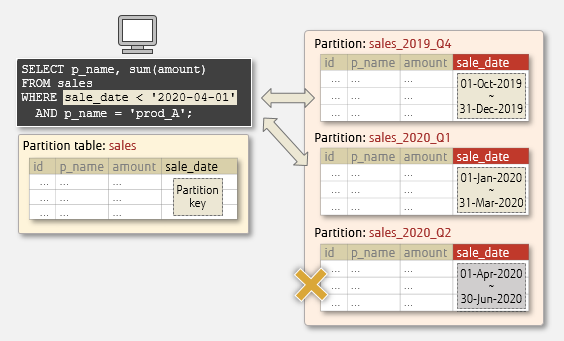
Partition pruning is a feature that narrows down the partitions to be accessed by SQLs, which in effect means you can exclude those that do not need to be scanned. In the partitioning overview article mentioned above, we explain how to specify a partition key to limit the search range - this is possible thanks to this partition pruning feature.

For example, in the figure below, the sale_date column is set as a partition key. By using the partition key in WHERE clause, the partitions to be accessed are narrowed down. Since the search is performed only for the targeted partitions, efficient scan is possible.

Pruning partitions

Note the following about partition pruning:

• They are enabled by default.
• They can be enabled/disabled by setting enable_partition_pruning in postgresql.conf or by using SET.

Partition pruning example

Let's see the effect of partition pruning by comparing the scan performance for partitioned and non-partitioned tables. The sales table in the sample below employs a range partition, with sale_date as the partition key. You can see that the table is divided into three partitions, while nonpartition_sales is not a partition table.

Partitioned table

mydb=# \d+ sales
    Table "public.sales"
  Column   |    Type    |…
-----------+------------+
 id        | integer    |
 p_name    | text       |
 amount    | integer    |
 sale_date | date       |
Partition key: RANGE (sale_date)

Partitions: sales_2019_Q4 FOR VALUES FROM ('2019-10-01') TO ('2020-01-01'),
            sales_2020_Q1 FOR VALUES FROM ('2020-01-01') TO ('2020-04-01'),
            sales_2020_Q2 FOR VALUES FROM ('2020-04-01') TO ('2020-07-01')

mydb=# SELECT COUNT(*) FROM sales;
  count
---------
 3000000
(1 row)

Non-partitioned table

mydb=# \d+ nonpartition_sales
    Table "public.nonpartition_sales"
  Column   |    Type    |…
-----------+------------+
 id        | integer    |
 p_name    | text       |
 amount    | integer    |
 sale_date | date       |

mydb=# SELECT COUNT(*) FROM nonpartition_sales;
  count
---------
 3000000
(1 row)

Comparing estimated execution times

Let's check the execution plan in the non-partitioned table of a SELECT statement using the partition key (sale_date).

mydb=# EXPLAIN ANALYZE SELECT * FROM nonpartition_sales
mydb-# WHERE sale_date < '2020-04-01' AND id=1;
                        QUERY PLAN
------------------------------------------------------------
 Gather …
  Workers Planned: 2
  Workers Launched: 2
  -> Parallel Seq Scan on nonpartition_sales A …
      Filter: ((sale_date < '2020-04-01'::date) AND (id = 1))
      Rows Removed by Filter: 986797
 Planning Time: 0.249 ms
 Execution Time: 3156.240 ms B
(8 rows)

Now let's see how the plan changes when executing the same SQL for the partitioned table.

mydb=# EXPLAIN ANALYZE SELECT * FROM sales
mydb-# WHERE sale_date < '2020-04-01' AND id=1;
                        QUERY PLAN
----------------------------------------------------------------
 Gather …
  Workers Planned: 2
  Workers Launched: 2
  -> Parallel Append …
     -> Parallel Seq Scan on sales_2019_Q4 A …
         Filter: ((sale_date < '2020-04-01'::date) AND (id = 1))
         Rows Removed by Filter: 292428
     -> Parallel Seq Scan on sales_2020_Q1 A …
         Filter: ((sale_date < '2020-04-01'::date) AND (id = 1))
         Rows Removed by Filter: 539199
 Planning Time: 0.642 ms
 Execution Time: 423.267 ms B
(12 rows)

As we can see above, the execution time for the partitioned table is almost 7.5x faster (3,156.240 ms x 423.267ms).

Partition-wise join

Partition-wise join is a feature that joins partitions during a JOIN operation on partitioned tables. Combining partitions that have the same range and values eliminates unnecessary JOIN processing, thus improving performance.

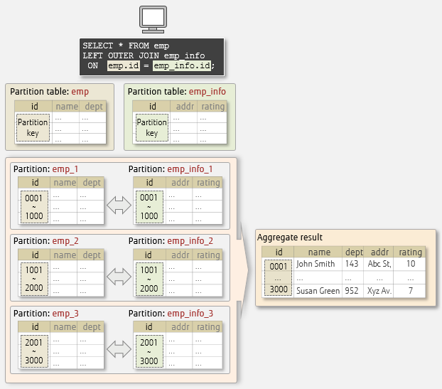
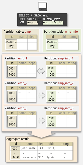
Let's look at an example in the diagram below, where both the emp and the emp_info tables are partitioned, with the id column of each table set as the partition key, and both tables have the same range partitioning - values 1 to 1000, 1001 to 2000, and 2001 to 3000.

Our JOIN condition is emp.id = emp_info.id, so the emp_1 and the emp_info1 partitions are joined, since they meet the join condition (each id column takes values from 1 to 1000). However, the emp_1 and the emp_info_2 partitions do not join, since they have been partitioned with different values. Other partitions created with the same partitioning range values are also joined, as illustrated below.

Aggregating partitions – JOIN

Aggregating partitions

Note the following about partition-wise joins:

• They are disabled by default. This is because a lot of CPU and memory may be consumed when creating execution plans. Verification is required whether they will be effective in your environment before using them.
• They can be enabled/disabled by setting enable_partitionwise_join in postgresql.conf or by using SET.
• Their performance may be even amplified by using parallel query - we will discuss this later in this article.

Partition-wise join example

Let's compare the estimated times in execution plans where partition-wise joins are disabled and enabled.

The emp and emp_info tables in this example uses hash partitioning, with the id column set as the partition key. Both tables are divided into 3 partitions under the same conditions.

Table emp

mydb=# \d+ emp
      Table "public.emp"
 Column |  Type   | …
--------+---------+
 id     | integer |
 name   | text    |
 dept   | integer |
Partition key: HASH (id)
Index:
  "emp_pkey" PRIMARY KEY, btree (id)
Partition: emp_0 FOR VALUES WITH (modulus 3, remainder 0),
           emp_1 FOR VALUES WITH (modulus 3, remainder 1),
           emp_2 FOR VALUES WITH (modulus 3, remainder 2)

mydb=# SELECT COUNT (*) FROM emp;
  count
---------
 3000000
(1 row)

Table emp_info

mydb=# \d+ emp_info
      Table "public.emp_info"
 Column |  Type   | …
--------+---------+-
 id     | integer | 
 addr   | text    | 
 rating | integer | 
Partition key: HASH (id)
Index:
  "emp_pkey" PRIMARY KEY, btree (id)
Partition: emp_info_0 FOR VALUES WITH (modulus 3, remainder 0),
           emp_info_1 FOR VALUES WITH (modulus 3, remainder 1),
           emp_info_2 FOR VALUES WITH (modulus 3, remainder 2)

mydb=# SELECT COUNT (*) FROM emp_info;
  count
---------
 3000000
(1 row)

Comparing estimated execution times

mydb=# SHOW enable_partitionwise_join;
  enable_partitionwise_join
-------------------------------------
off
(1 row)

mydb=# EXPLAIN ANALYZE
mydb-# SELECT emp.id, emp.name, emp_info.rating
mydb-#   FROM emp LEFT OUTER JOIN emp_info
mydb-#     ON emp.id = emp_info.id A
mydb-#   WHERE emp_info.rating = 10;
                   QUERY PLAN
---------------------------------------------------
Gather …
 Workers Planned: 2
 Workers Launched: 2
 -> Parallel Hash Join …
     Hash Cond: (emp_1.id = emp_info_1.id)
     -> Parallel Append B …
         -> Parallel Seq Scan on emp_1 …
         -> Parallel Seq Scan on emp_0 …
         -> Parallel Seq Scan on emp_2 …
     -> Parallel Hash …
         -> Parallel Append C …
             -> Parallel Seq Scan on emp_info_1 …
                 Filter: (rating = 10)
                 Rows Removed by Filter: 326749
             -> Parallel Seq Scan on emp_info_0 …,
                 Filter: (rating = 10)
                 Rows Removed by Filter: 980068
             -> Parallel Seq Scan on emp_info_2 …
                 Filter: (rating = 10)
                 Rows Removed by Filter: 489780
 Planning Time: 0.538 ms
 Execution Time: 11080.809 ms D
(23 rows)

mydb=# SET enable_partitionwise_join TO on;
SET
mydb=# SHOW enable_partitionwise_join;
  enable_partitionwise_join
----------------------------
on
(1 row)

mydb=# EXPLAIN ANALYZE
mydb-# SELECT emp.id, emp.name, emp_info.rating
mydb-#   FROM emp LEFT OUTER JOIN emp_info
mydb-#     ON emp.id = emp_info.id A 
mydb-# WHERE emp_info.rating = 10;
                 QUERY PLAN
-------------------------------------------------
Gather …
 Workers Planned: 2
 Workers Launched: 2
 -> Parallel Append …
     -> Nested Loop …
         -> Parallel Seq Scan on emp_info_1 B …
             Filter: (rating = 10)
             Rows Removed by Filter: 980248
         -> Index Scan using emp_1_pkey on emp 1 C …
             Index Cond: (id = emp_info_1.id)
     -> Nested Loop …
         -> Parallel Seq Scan on emp_info_0 …
             Filter: (rating = 10)
             Rows Removed by Filter: 980068
         -> Index Scan using emp_0_pkey on emp0 …
             Index Cond: (id = emp_info_0.id)
     -> Nested Loop …
         -> Parallel Seq Scan on emp_info_2  …
             Filter: (rating = 10)
             Rows Removed by Filter: 326520
         -> Index Scan using emp_2_pkey on emp_2 …
             Index Cond: (id = emp_info_2.id)
 Planning Time: 1.290 ms
 Execution Time: 1136.806 ms D 
(25 rows)

As we can see above, the execution time using partition-wise join is almost 10x faster (11,080. 809 ms x 1,136.806 ms).

The Nested Loop makes a big difference in speed because the data range to scan during the join processing of partitions is reduced.

The execution plan changes depending on whether partition-wise join is enabled. With this feature, you can optimise JOIN by filtering the scan target in the most efficient way.

Partition-wise aggregation

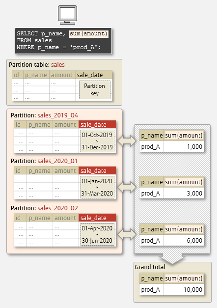
In partition-wise aggregation, aggregation is done for each partition in a partition table and the results are integrated at the end. Processing time can be shortened by performing aggregation for each partition.

For example, in the following figure, aggregation is processed for each partition, and the results are integrated in the end.

Individual partition aggregation

Similarly to partition-wise joins, note the following about partition-wise aggregations:

• They are disabled by default. This is because a lot of CPU and memory may be consumed when creating execution plans. Verification is required whether they will be effective in your environment before using them.
• They can be enabled/disabled by setting enable_partitionwise_aggregate in postgresql.conf or by using SET.
• Their performance may be even amplified by using parallel query. Continue reading for an explanation of parallel query.

Partition-wise aggregation example

Again, let's compare the estimated times in execution plans for the same SQL statement, where partition-wise aggregation is disabled against after it is enabled.

The sales table in the example uses range partitioning, with sale_date set as the partition key. The table is divided into three partitions.

Table sales

mydb=# \d+ sales
  Table "public.sales"
 Column    |  Type   | …
-----------+---------+
 id        | integer |   
 p_name    | text    |   
 amount    | integer |   
 sale_date | date    |   
Partition key: RANGE (sale_date)
Index:
  "sales_id_idx" btree (id)
Partitions: sales_2019_Q4 FOR VALUES FROM ('2019-10-01') TO ('2020-01-01'),
            sales_2020_Q1 FOR VALUES FROM ('2020-01-01') TO ('2020-04-01'),
            sales_2020_Q2 FOR VALUES FROM ('2020-04-01') TO ('2020-07-01')

mydb=# SELECT COUNT (*) FROM sales;
  count
---------
 3000000
(1 row)

Comparing estimated execution times

mydb=# SHOW enable partitionwise_aggregate;
 enable_partitionwise_aggregate
------------------------------
off
(1 row)

mydb=# EXPLAIN ANALYZE
mydb-# SELECT p_name, sum(amount) sales_total FROM sales
mydb-# WHERE p_name = 'prod_A' GROUP BY p_name;
                QUERY PLAN
-----------------------------------------------------------
GroupAggregate …
  Group Key: sales_2019_Q4.p_name
  -> Append …
     -> Bitmap Heap Scan on sales_2019_Q4  A …
         Recheck Cond: (p_name = 'prod_A'::text)
         Heap Blocks: exact=5483
         -> Bitmap Index Scan on sales_2019_Q4_p_name_idx …
             Index Cond: (p_name = 'prod_A'::text)
     -> Bitmap Heap Scan on sales_2020_Q1  A …
         Recheck Cond: (p_name = 'prod_A'::text)
         Heap Blocks: exact=6716
         -> Bitmap Index Scan on sales_2020_Q1_p_name_idx …
             Index Cond: (p_name = 'prod_A'::text)
     -> Bitmap Heap Scan on sales_2020_Q2  A …
         Recheck Cond: (p_name = 'prod_A'::text)
         Heap Blocks: exact=6120
         -> Bitmap Index Scan on sales_2020_Q2_p_name_idx …
             Index Cond: (p_name = 'prod_A'::text)
 Planning Time: 0.345 ms
 Execution Time: 503.067 ms B
(20 rows)

mydb=# SET enable_partitionwise_aggregate TO on;
SET
mydb= SHOW enable partitionwise aggregate;
 enable_partitionwise_aggregate
--------------------------------
on
(1 row)

mydb=# EXPLAIN ANALYZE
mydb-# SELECT p_name, sum(amount) sales_total FROM sales
mydb)# WHERE p_name = 'prod_A' GROUP BY p_name;
                    QUERY PLAN
--------------------------------------------------------
 Finalize GroupAggregate …
  Group Key: sales_2019_Q4.p_name
   -> Append …
      -> Partial GroupAggregate …
          Group Key: sales_2019_Q4.p_name A
          -> Bitmap Heap Scan on sales_2019_Q4 …
              Recheck Cond: (p_name = 'prod_A'::text)
              Heap Blocks: exact=5483
              -> Bitmap Index Scan on sales_2019_Q4_p_name_idx …
                  Index Cond: (p_name = 'prod_A'::text)
      -> Partial GroupAggregate …
          Group Key: sales_2020_Q1.p_name A
          -> Bitmap Heap Scan on sales_2020_Q1_p_name …
              Recheck Cond: (p_name = 'prod_A'::text)
              Heap Blocks: exact=6716
              -> Bitmap Index Scan on sales_2020_Q1_p_name_idx …
                  Index Cond: (p_name = 'prod_A'::text)
      -> Partial GroupAggregate …
          Group Key: sales_2020_Q2.p_name A
          -> Bitmap Heap Scan on sales_2020_Q2 …
              Recheck Cond: (p_name = 'prod_A'::text)
              Heap Blocks: exact=6120
              -> Bitmap Index Scan on sales_2020_Q2_p_name_idx …
                  Index Cond: (p_name = 'prod_A'::text)
 Planning Time: 0.522 ms
 Execution Time: 394.091 ms B 
(26 rows)

As we can see above, the execution time using partition-wise aggregation is almost 30% faster (503.067ms x 394.091ms) - this is because the number of target rows is reduced by executing aggregation in each partition – with fewer rows to scan, the overall speed is increased.

Parallel query for partition table

Parallel query is a feature that executes a single SQL in parallel using multiple processes. Performance is improved because the processing is distributed to multiple CPUs.

Parallel queries can be executed on partition tables, allowing performance benefits of partition-wise joins and partition-wise aggregations to be enhanced even further. This is due to the fact that processing is carried out in parallel for each partition, with the results then combined at the end.

In the example below where we query a partitioned table, we see that a sequential scan is performed on each partition in parallel.

mydb=# EXPLAIN SELECT COUNT(*) FROM sales;
                   QUERY PLAN
-----------------------------------------------------
Finalize Aggregate …
 -> Gather …
     Workers Planned: 2
     -> Partial Aggregate …
         -> Parallel Append …
             -> Parallel Seq Scan on sales_2020_Q2 …
             -> Parallel Seq Scan on sales_2020_Q1 …
             -> Parallel Seq Scan on sales_2019_Q4 …
(8 rows)

Parallel queries in partitioned tables are enabled by default. They can be enabled/disabled by setting enable_parallel_append in postgresql.conf.

In this article, we explained how performance can be improved with PostgreSQL partitioning features. Always remember that it is important to thoroughly understand how these features work before using them in your system.