What is partitioning?

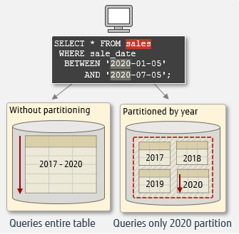
A table can be partitioned according to the conditions you specify. Therefore, it is necessary to set optimum conditions considering the data characteristics and the purpose of use. With partitioning, the table is split into smaller groups based on the specified criteria, but can still be treated as one table from the application. The image of partitioning is shown below.

Execution with/without partitioning

Benefits of partitioning

Partitioning can provide improved performance and maintainability. Let's have a look at these benefits.

Improved performance

By splitting the table, search performance is enhanced – the contributing factors are listed below:

• I/O reduction due to table partitioning
  By specifying the search condition in SQL, the access range can be narrowed down to a specific partition. It also makes it easier for frequently used parts of the partition to be cached in memory. In addition, this reduces disk I/O and improves access performance.
• I/O distribution by spreading into different tablespaces
  The partitioned table can be placed in different tablespaces on physical disks. This distributes disk I/O, with reads and writes being performed in parallel on different physical disks, thus improving performance.

Improved maintainability

Data can be added, deleted, and updated for each partition, improving maintainability in operation. For example, when using a system that retains sales data for 5 years in monthly partitions, it is possible to create a new partition when the month changes, and delete the same month partition from 5 years ago. In addition, the partitioned data can be deleted using DROP TABLE or TRUNCATE. Both can speed up the deletion processing and reduce the VACUUM load compared to the data deletion by DELETE.

Partition types supported by PostgreSQL

You need to specify the column (called partition key) to be used for partitioning – values in this column will be used to create partitions. Depending on how you would like to group your data, different types of partitioning are available. PostgreSQL supports the partitioning methods below – select the appropriate one according to your business needs and operation.

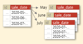
Range partitioning

• Data is partitioned according to the specified range.

• Effective when you want to access time-series data, by specifying date such as year and month.

• Example: Split by sale date, admission date, etc.

Partitioning by date range

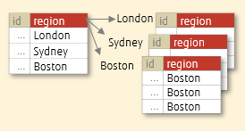
List partitioning

• Data is partitioned according to the specified discrete values.

• Effective when you want to group discrete data, such as regions and departments with arbitrary values.

• Example: Split by region, job title, etc

Partitioning by region

Hash partitioning

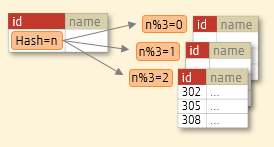
• Data is partitioned by specifying a modulus and a remainder for each partition. Each partition will hold the rows for which the hash value of the partition key divided by the modulus will produce the specified remainder.

• Effective when you want to avoid access concentration to a specific table by distributing data almost evenly.

• Example: Split into 3 partitions (n is the hash value created from the value in the partition key)
  • n % 3 = 0 → Allocates to partition 1
  • n % 3 = 1 → Allocates to partition 2
  • n% 3 = 2 → Allocates to partition 3

Partitioning by id hash

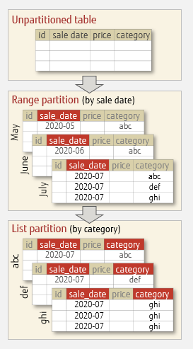
It is also possible to create additional partitions under a partition, as shown below, to create a more detailed partition setup. This setup is called a composite partition, or subpartition.
For example, for the product sales table (partition table), you can create a range partition divided by month, and underneath that, create a list partition divided by product category. Access performance is improved because you can narrow down the partitions to be searched, such as when you want to retrieve the sales data of a specific product category in a particular time period (for example, sales data for product category 'ghi' in July).

Composite partition setup

How to use partitioning

Let's see how partitioning works with a simple example. The database used in the sample is 'mydb'.

How to create a partition table

To create a partition table, first use CREATE TABLE, specifying the partition type and partition key. Then create each partition, using CREATE TABLE as well, specifying the partitioning method.

Creating a range partition

Sample scenario: Create a partition table containing daily sales split per quarter.

1Create the partition table.

mydb=# CREATE TABLE sales (id int, p_name text, amount int, sale_date date)
mydb-# PARTITION BY RANGE (sale_date);

2Create the partitions.

mydb=# CREATE TABLE sales_2019_Q4 PARTITION OF sales FOR VALUES FROM ('2019-10-01') TO ('2020-01-01');
mydb=# CREATE TABLE sales_2020_Q1 PARTITION OF sales FOR VALUES FROM ('2020-01-01') TO ('2020-04-01');
mydb=# CREATE TABLE sales_2020_Q2 PARTITION OF sales FOR VALUES FROM ('2020-04-01') TO ('2020-07-01');

3Add data to the partition table.

mydb=# INSERT INTO sales VALUES (1,'prod_A',100,'2020-06-01');
mydb=# INSERT INTO sales VALUES (8,'prod_B', 5,'2020-03-02');
…

4Retrieve data from the partition table.

mydb=# SELECT * sales;
 id | p_name | amount | sale_date
----+--------+--------+------------
  1 | prod_A |    100 | 2020-06-01
  8 | prod_B |      5 | 2020-03-02 
  2 | prod_F |     15 | 2020-03-02
  3 | prod_B |      5 | 2020-01-15
  4 | prod_C |     10 | 2020-02-11
  6 | prod_F |     10 | 2020-01-05
 10 | prod_E |      5 | 2020-02-10
  5 | prod_E |     10 | 2020-05-15
  7 | prod_D |     10 | 2020-04-11
  9 | prod_C |     15 | 2020-04-30
(10 rows)

5Retrieve data from a partition.

mydb=# SELECT * FROM sales_2020_Q2;
 id | p_name  | amount | sale_date
----+---------+--------+------------
  5 | prod_E  |     10 | 2020-05-15
  7 | prod_D  |     10 | 2020-04-11
  9 | prod_C  |     15 | 2020-04-30
(3 rows)

Creating a list partition

Sample scenario: Using the table that manages sales of each branch office, create a list partition that divides the table by region.

1Create the partition table.

mydb=# CREATE TABLE sales_region (id int, amount int, branch text, region text)
mydb-# PARTITION BY LIST (region);

2Create the partitions.

mydb=# CREATE TABLE London PARTITION OF sales_region FOR VALUES IN ('London');
mydb=# CREATE TABLE Sydney PARTITION OF sales_region FOR VALUES IN ('Sydney');
mydb=# CREATE TABLE Boston PARTITION OF sales_region FOR VALUES IN ('Boston');

3Add data to the partition table.

mydb=# COPY sales_region FROM '/home/tmp/listpart_1.sql';

4Retrieve data from the partition table.

mydb=# SELECT * FROM sales_region;
  id | amount |  branch    | region
-----+--------+------------+--------
 136 |    150 |   Kings Rd | London
 147 |     10 |  Regent St | London
 245 |    100 | College St | Sydney
 278 |     50 |  George St | Sydney
 561 |    100 | Charles St | Boston
 537 |      5 |     Ann St | Boston
 510 |     10 |    Park Dr | Boston
(7 rows)

5Retrieve data from a partition.

mydb=# SELECT * FROM Boston;
  id | amount |  branch    | region
-----+--------+------------+--------
 561 |    100 | Charles St | Boston
 537 |      5 |     Ann St | Boston
 510 |     10 |    Park Dr | Boston
(3 rows)

Creating a hash partition

Sample scenario: Create a hash partition that evenly divides 1,000 pieces of data into 3 partitions.

In hash partitioning, hash values are created for the values of the partition key. That value is then divided by the number specified during creation of the partition - the remainder value of the calculation is used to determine the partition where the data should be stored. So, you need to specify the value to divide the hash value by, and also remainder value used to assign the row to a partition.

1Create the partition table.

mydb=# CREATE TABLE emp (emp_id int, emp_name text, dep_code int)
mydb-# PARTITION BY HASH (emp_id);

2Create the partitions.

mydb=# CREATE TABLE emp_0 PARTITION OF emp FOR VALUES WITH (MODULUS 3,REMAINDER 0);
mydb=# CREATE TABLE emp_1 PARTITION OF emp FOR VALUES WITH (MODULUS 3,REMAINDER 1);
mydb=# CREATE TABLE emp_2 PARTITION OF emp FOR VALUES WITH (MODULUS 3,REMAINDER 2);

3Add data to the partition table.

mydb=# INSERT INTO emp SELECT num,
mydb-# 'user_' || num , (RANDOM()*50)::INTEGER FROM generate_seriesx(1,1000) AS num;

4Check the number of rows in the partition table and each partition

mydb=# SELECT relname,reltuples as rows FROM pg_class
mydb-# WHERE relname IN ('emp','emp_0','emp_1','emp_2')
mydb-# ORDER BY relname;
 relname | rows
---------+--------
 emp     |    0
 emp_0   |  324 A
 emp_1   |  333
 emp_2   |  343
(4 rows)

Creating a default partition for out-of-range date

For range and list partitions you can also create a default partition for storing out-of-range data, that is, data that does not satisfy any of the defined split conditions. A default partition allows you to temporarily store out-of-range data, so that at a later time you can create a partition to store it.

Trying to insert out-of-range data in a table without default partition will result in error.

Assuming we have the table sales_region list-partitioned by region as follows:

mydb=# \d+ sales_region
       table "public.sales_region"
 Column |  Type    …
--------+-----------
id      | integer  
amount  | integer  
branch  | text     
region  | text     
Partition key: LIST (region)
Partition: London FOR VALUES IN ('London'),
           Sydney FOR VALUES IN ('Sydney'),
           Boston FOR VALUES IN ('Boston')

1Create the default partition.

mydb=# CREATE TABLE region_default PARTITION OF sales_region DEFAULT;

2Retrieve partition table information - the default partition will be displayed.

mydb=# \d+ sales_region
       table "public.sales_region"
 Column |  Type   …
--------+---------
id      | integer 
amount  | integer
branch  | text    
region  | text    
Partition key: LIST (region)
Partition: London FOR VALUES IN ('London'),
           Sydney FOR VALUES IN ('Sydney'),
           Boston FOR VALUES IN ('Boston'),
           region_default DEFAULT

3Insert out-of-range data into the partition table.

mydb=# INSERT INTO sales_region VALUES(11, 10, 'Bourke St', 'Quebec');
INSERT 0 1

4Retrieve data from the default partition.

mydb=# SELECT * FROM region_default;
 id | amount |  branch   | region
----+--------+-----------+--------
 11 |     10 | Bourke St | Quebec
(1 row)

Partitioning behavior

Let's have a look at how users carry out their operations in partition tables, and how PostgreSQL handles them.

Searching a partition table

mydb=# SELECT * FROM emp WHERE emp_id=1000;
 emp_id  | emp_name  | dep_code
---------+-----------+-----------
    1000 | user_1000 |        7
(1 row)

mydb=# EXPLAIN ANALYZE SELECT * FROM emp WHERE emp_id=1000;
                       QUERY PLAN
-----------------------------------------------------------
 Append ...
   ->  Seq Scan on emp_2 …
        Filter: (emp_id = 1000)
         Rows Removed by Filter: 342
 Planning Time: 0.293 ms
 Execution Time: 0.101 ms
(6 rows)

Updating data between partitions

When the value in the partition key column is updated, the relevant data is moved to the appropriate partition automatically.

We can check this with the steps below - in the following example, we move the Park Dr branch row from the Boston partition to the London partition.

1Retrieve data from the Boston partition, which includes the Park Dr branch.

mydb=# SELECT * FROM Boston;
  id | amount |  branch    | region A
-----+--------+------------+---------
 561 |    100 | Charles St | Boston
 537 |      5 |     Ann St | Boston
 510 |     10 |    Park Dr | Boston
(3 rows)

2Change the region of branch 'Park Dr' from Boston to London.

mydb=# UPDATE sales_region
mydb-# SET region='London' WHERE branch='Park Dr';

3Retrieve data from the London partition, which now includes the Park Dr branch.

mydb=# SELECT * FROM London;
  id | amount |   branch   |  region
-----+--------+------------+---------
 136 |    150 |   Kings Rd | London
 147 |     10 |  Regent St | London
 510 |     10 |    Park Dr | London
(4 rows)

Adding a partition

When performance cannot be expected to improve with the current number of partitions due to an increase in the amount of data, it may be desirable to increase the number of partitions, to create a more detailed partition setup for enhanced performance.

The number of range partitions and list partitions can be increased by specifying a new range and value for the partition key. However, hash partitions cannot be added in the same way, because the number of partitions is determined by division calculation and specified remainder values. Let's look at an example of repartitioning a hash partition by updating the value to be used for division and the remainder values. Here, the hash partition created above is used as a sample.

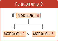
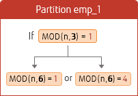
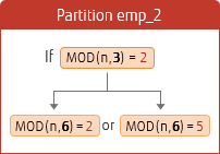
Specify the multiple number of the current value set for division calculation. The following is an example of changing the hash partition from 3 partitions to 6 partitions (a multiple of 3).

Based on the above, we will explain the procedure to divide into 6 partitions. We assume that the partition table contains 1 million rows, and that they are split into the partitions as follows.

mydb=# SELECT relname, reltuples as rows FROM pg_class
mydb-# WHERE relname IN ('emp','emp_0','emp_1','emp_2')
mydb-# ORDER BY relname;
 relname | rows
---------+--------
 emp     |      0
 emp_0   | 333263 A
 emp_1   | 333497
 emp_2   | 333240
(4 rows)

1Detach the partitions from the partition table.

mydb=# ALTER TABLE emp DETACH PARTITION emp_0;
mydb=# ALTER TABLE emp DETACH PARTITION emp_1;
mydb=# ALTER TABLE emp DETACH PARTITION emp_2;

2Rename the partitions.

mydb=# ALTER TABLE emp_0 RENAME TO emp_0_bkp;
mydb=# ALTER TABLE emp_1 RENAME TO emp_1_bkp;
mydb=# ALTER TABLE emp_2 RENAME TO emp_2_bkp;

3Create six partitions.

mydb=# CREATE TABLE emp_0 PARTITION OF emp FOR VALUES WITH (MODULUS 6, REMAINDER 0);
mydb=# CREATE TABLE emp_1 PARTITION OF emp FOR VALUES WITH (MODULUS 6, REMAINDER 1);
mydb=# CREATE TABLE emp_2 PARTITION OF emp FOR VALUES WITH (MODULUS 6, REMAINDER 2);
mydb=# CREATE TABLE emp_3 PARTITION OF emp FOR VALUES WITH (MODULUS 6, REMAINDER 3);
mydb=# CREATE TABLE emp_4 PARTITION OF emp FOR VALUES WITH (MODULUS 6, REMAINDER 4);
mydb=# CREATE TABLE emp_5 PARTITION OF emp FOR VALUES WITH (MODULUS 6, REMAINDER 5);

4Restore the data from the detached partitions.

mydb=# INSERT INTO emp SELECT * FROM emp_0_bkp;
mydb=# INSERT INTO emp SELECT * FROM emp_1_bkp;
mydb=# INSERT INTO emp SELECT * FROM emp_2_bkp;

5Delete the detached partitions.

mydb=# DROP TABLE emp_0_bkp;
mydb=# DROP TABLE emp_1_bkp;
mydb=# DROP TABLE emp_2_bkp;

6The data was divided into six partitions as shown below.

mydb=# SELECT relname,reltuples as rows FROM pg_class
mydb-# WHERE relname IN ('emp','emp_0','emp_1','emp_2','emp_3','emp_4','emp_5')
mydb-# ORDER BY relname;
 relname | rows
---------+---------
 emp     |       0
 emp_0   |  166480 A
 emp_1   |  166904
 emp_2   |  166302
 emp_3   |  166783
 emp_4   |  166593
 emp_5   |  166938
(7 rows)

Performing the steps above for all partitions at once may take time if the amount of data is large. In such a case, you can perform the steps separately for each partition. You can choose the optimum partitioning range according to the amount of data and operation.

In this article, we outlined major partitioning methods using practical examples. You can expect improved performance and maintainability by implementing partitioning and splitting tables according to your business and operation.