SQL tuning involves an analysis of execution plans and tweaking of time-consuming SQLs to optimize the system performance. In this article, we use a sample to perform tuning to show you the overall flow of SQL tuning.
How tables are scanned and joined
In SQL tuning, the SQL execution plan needs to be analyzed. Before we jump into SQL tuning, we will briefly go over how tables are scanned and joined, the logic of which analysis of the execution plan will be based on.
Scanning method
How are tables accessed? The following are the major scanning methods.
- Sequential Scan
Accesses tables sequentially from start to finish. This is an effective method when a large number of items need to be retrieved.
- Index Scan
Accesses indexes and tables alternately. This is an effective method when the number of items to be retrieved using the WHERE clause is small or when you want to access a specific data.
Join method
How are two tables joined? From the scan results of two tables, one result is output. The following are the major join methods. To distinguish the two tables to be joined, they are called outer table and inner table.
- Nested Loop Join
Nested Loop Join
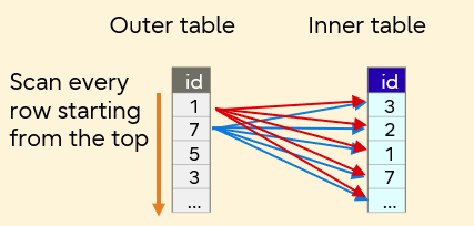
This method joins the inner table by looping all inner table rows for each outer table row. Processing is accelerated when the outer table has a small number of rows and the inner table has an index.
- Merge Join
Merge Join
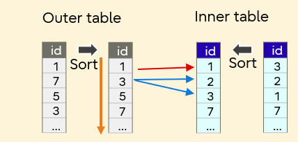
This is a method to sort two tables by a join key and then join them in sequence. This method is not efficient if sort takes a long time. Processing is accelerated because by defining a primary key or an index as the join key, the sort results of the two tables can be matched. This is an effective method when joining large tables.
- Hash Join
Hash Join
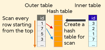
This is a method to create a hash with the join key of the inner table and join the hash by matching against the rows of the outer table. The hash is created in memory, so once created, join is processed at a high speed. However, if the hash is larger than the memory size, file access will occur, resulting in slow processing. This method is suitable to join relatively small tables with large tables.
Detecting slow SQL
Slow SQLs can be detected via statistics views and server logs.
Using statistics view
Execute the following SQL to the pg_stat_statements view, and output 3 long-running SQLs in order from the slowest (for PostgreSQL version older than 13, replace total_exec_time with total_time).
SELECT query, calls, CAST(total_exec_time as numeric(10,3)), CAST(total_time/calls AS numeric(10,3)) AS avg_time
FROM pg_stat_statements ORDER BY avg_time DESC,calls LIMIT 3;
The output will be something like the following:
query | calls | total_time | avg_time
-----------------------------------------------------------------------+-------+------------+-----------
SELECT sales.name,sum(sales.num),(sum(sales.num)) * price.price | 5 | 31000.071 | 6200.014
AS total_price FROM sales,price WHERE sales.name = price.name | | |
GROUP BY sales.name.price.price ORDER BY sales.name ASC | | |
SELECT sales.name,sum sales.num,sum(sales.num) * price.price | 2 | 5886.436 | 2943.218
AS total_price FROM sales,price WHERE sales.name = price.name | | |
AND sales.datetime BETWEEN $1 AND $2 GROUP BY sales.name,price.price | | |
SELECT sales.name,sum(sales.num) AS sum FROM sales GROUP BY sales.name | 6 | 6793.545 | 1132.257
(3 rows)
From pg_stat_statements view, you can see that the SQL that searches the sales and price tables is taking time.
Refrence
In addition to query statistics (pg_stat_statements), planner statistics (pg_statistic) and function statistics (pg_stat_user_functions) can be obtained periodically to use for analysis when performance deterioration occurs.
Checking the server log
In the example statistics output above, we have identified a SQL that takes 6 seconds on average. Next, we will check for SQLs that takes more than 3 seconds, using the server log (by setting the log_min_duration_statement parameter in postgresql.conf to 3 seconds).
00000: 2019-03-05 11:18:08 JST [11408]: (3-1) user = fsep,db = mydb,remote = ::1(50650) app = psql
LOG: duration: 6518.096 ms statement: SELECT sales.name, sum(sales.num),(sum(sales.num)) * price. price
AS total_price FROM sales,price WHERE sales.name = price.name GROUP BY sales.name,price.price
ORDER BY sales.name ASC;
000000: 2019-03-05 11:21:30 JST [7184]: [7-1] user = ,db = ,remote = app = LOG: checkpoint starting: time
000000: 2019-03-05 11:21:32 JST [7184]: [8-1] user = ,db = ,remote = app = LOG: checkpoint complete: wrote
14 buffers (0.0%); O WAL file(s) added, 0 removed, 6 recycled; write=1.556 s, sync=0.014 s, total=1.693 s;
sync files=13, longest=0.001 s, average=0.001 s; distance=199525 kB, estimate=199525 kB
You can see that the SQL that looks up the sales and price tables takes a long time to execute, as also confirmed in the statistics view.
Reference
In the server log, you can check the duration for each SQL, as well as the calling user (user), database (db), application (app), etc. However, settings must be done in advance for parameters including log_min_duration_statement and log_line_prefix in postgresql.conf so that this information is output to the log.
Investigation
Let's find out why processing search on the sales and price tables take time.
Viewing the execution plan
First, execute EXPLAIN to check the execution plan of the target SQL and investigate what is causing the problem. Then, execute the SQL with ANALYZE to check the actual measurement value. Remember, ANALYZE actually executes the SQL statement. When displaying execution plans for commands including INSERT and DELETE, use BEGIN and ROLLBACK statements to avoid affecting the data.
mydb=# EXPLAIN ANALYZE SELECT sales.name,sum(sales.num),(sum(sales.num)) * price.price AS total FROM sales, pri
ce WHERE sales.name = price.name GROUP BY sales.name,price.price ORDER BY Sales.name ASC;
QUERY PLAN
----------------------------------------------------------------------------------------------------------------
Sort (cost=853626.74..853626.89 rows=60 width=26) (actual time=16518.220..16518.223 rows=10 loops=1)
Sort Key: sales.name
Sort Method: quicksort Memory: 25kB
-> HashAggregate (cost=853624.21..853624.96 rows=60 width=26) (actual time=16518.195..16518.200 rows=10
loops=1).
Group Key: sales.name, price.price
Merge Join1 (cost=728623.09..803624.30 rows=49999914 width=14) (actual time=6149.953..13546.6562
rows=50000004 loops=1)
Merge Cond: ((sales.name)::text = (price.name) ::t
-> Sort (cost=728553.76..741053.74 rows=4999991 width=10) (actual time=6148.266..8810.2902
rows=5000000 loops=1)
Sort Key: sales.name
Sort Method: external merge Disk: 108648KB2
-> Seq Scan on sales3 (cost0.00..86764.91 rows=49999914 width=10)
actual time=0.028..2540.105 rows=50000004 loops=1)
-> Sort (cost=65.83..68.33 rows=1000 width=13) (actual time=1.161..1.529 rows=963 loops=1)
Sort Key : price.name
Sort Method: quicksort Memory: 74KB5
-> Seq Scan on price3 (cost=0.00..16.00 rows=10004 width=13) (actual time=0.020..0.445
rows=10004 loops=1)
Planning time: 0.327 ms
Execution time: 16529.869 ms
(17 rows)
From the execution plan, we can tell that the final execution time is 16529.869ms, and the following can also be observed.
1"Merge Join" is selected as the method of joining the sales and price tables.
2The sort method of the sales table is "external sort (external merge: writes the sort result to an external file)", which takes considerable time. As a result, the entire merge join takes significant time.
3"Seq Scan" is selected as the scan method for the sales and price tables.
4Statistics are up to date, because the number of rows for the estimated and measured values are almost the same.
5In the price table, "quicksort (in-memory sort)" is selected, so it is processed at high speed in memory (used 74kB).
To identify a tuning point, refer to the actual time to see which processing is taking a long time. As you can see, there are no particular problems with 4 and 5 above, but the join in 1, 2, and 3 are taking a long time. This means we need to review whether the merge join method is appropriate, and whether the process can be improved.
Reference
In 2, external sort is used because the memory used for sort exceeds the value of the work_mem parameter of postgesql.conf. In this case, one solution is to specify a value larger than the disk (108648kB) to the work_mem parameter as described below and change the sort method to quicksort which speeds up the process.
- Modify postgesql.conf on the server
- Change the value using PGOPTIONS on the client
- Change the value using set on the client
If you modify postgresql.conf on the server, the changes will take effect for the entire database cluster. This means significant increase of memory usage. For this reason, make changes to the client side as much as possible to localize the impact.
Checking numbers of data records
The following shows the number of data records in sales table and price table.
mydb=# SELECT COUNT(*) FROM sales;
count
---------
5000000
(1 row)
mydb=# SELECT COUNT(*) FROM price;
count
---------
1000
(1 row)
The sales table has 5 million records, and the price table has 1000 records. In this case, the tables joined are both relatively large for the database environment, so it can be assumed that merge join is a reasonable join method.
Checking table definitions
Next, output the table definitions of sales table and price table to confirm the definition for "name", the join key specified as the condition of WHERE.
mydb=# ¥d sales
Table "public.sales"
Column | Type | Collation | Nullable | Default
------------+-----------------------------+------------+-------------+-------------------------------------
id | integer | | not null | nextval('sales_id_seq' :: regclass)
name | character varying (255) | | not null |
datetime | timestamp without time zone | | not null |
num | integer | | not null |
mydb=# ¥d price
Table "public.price"
Column | Type | Collation | Nullable | Default
------------+-----------------------------+------------+-------------+-------------------------------------
id | integer | | not null | nextval('price_id_seql' :: regclass)
name | character varying (255) | | not null |
price | integer | | not null |
Index:
"price_pkey" PRIMARY KEY, btree (name)
We can see that in the price table, the primary key column "name" is the index. However, even though the sales table is large, there is no index defined on the join key. We can presume that sorting takes long because no index is used for the join key in the merge join process.
Tuning
Based on the results described above (3. Investigation), add an index and check if the performance improves.
Adding an index
Add the index "sales_name_idx" to the column "name" of the sales table.
mydb=# CREATE INDEX sales_name_idx ON sales(name);
CREATË INDEX
mydb=# ANALYZE;
ANALYZE
mydb=# ¥d sales
Table "public.sales"
Column | Type | Collation | Nullable | Default
------------+-----------------------------+------------+-------------+-------------------------------------
id | integer | | not null | nextval('sales_id_seq'::regclass)
name | character varying(255) | | not null |
datetime | timestamp without time zone | | not null |
num | integer | | not null |
Index:
"sales_name_idx” btree (name)
Check the execution plan
Output the execution plan again.
mydb=# EXPLAIN ANALYZE SELECT sales.name, sum(sales.num), (sum(sales.num)) * price.price AS total FRON sales,pri
ce WHERE sales.name = price.name GROUP BY sales.name,price.price ORDER BY sales.name ASC;
QUERY PLAN
-----------------------------------------------------------------------------------------------------------------
Sort (cost=390122.04..390122.19 rows=60 width=26) (actual time=9975.664..9975.668 rows=10 loops=1)
Sort Key: sales.name
Sort Method: quicksort Memory: 25kB
-> HashAggregate (cost=390119.52..390120.27 rows=60 width=26)
(actual time=9975.640..9975.646 rows=10 loops=1)
Group Key: sales.name, price.price
-> Merge Join (cost=57.67..340119.59 rows=4999993 width=14)
(actual time=1.504..7972.011 rows=5000000 loops=1)
Merge Cond: ((sales.name)::text = (price.name) ::text)
-> Index Scan using sales name idx on sales (cost=0.43..277540.46 rows=4999993 width=10)
(actual time=0.066..3083.440 rows=5100000 loops=1)
-> Index Scan using price_pkey on price (cost=0.28..79.15 rows=1000 width=13)
(actual time=0.009..0.933 rows=963 loops=1)
Planning time: 0.929 ms
Execution time: 9975.771 ms
(11 rows)
The sort executed as a pre-process of merge join and its associated "Seq Scan" have changed to "Index Scan" using the index "sales_name_idx". As a result, the time required for merge join is reduced (with index: 13546.656ms, without index: 7972.011ms) which shortened the overall execution time (with index: 16529.869ms, without index: 9975.771ms).
The execution time of EXPLAIN ANALYZE may differ from the SQL execution time (duration) confirmed in "Checking the server log" (it was 6518.096ms). We can check the SQL execution time (duration) in the server log after tuning. Set the log_min_duration_statement parameter in postgresql.conf to 0 (output all).
00000: 2019-03-05 15:29:44 JST [11408]: [43-1] user = fsep, db = mydb, remote = ::1(50650) app = psql
LOG: duration: 1479.164 ms statement: SELECT sales.name,sum(sales.num),(sum(sales.num)) * price.price
AS total FROM sales,price WHERE sales.name = price.name GROUP BY sales.name,price.price
ORDER BY sales.name ASC;
The duration shown here is 1479.164ms, so you can also see on the server log that the SQL execution time is now shorter.
In this article, we explained SQL tuning through an actual example. If performance problems occur during SQL execution, analyze execution plans and perform tuning so that appropriate processing can be implemented.